Summary

Random forests is a machine learning (ML) algorithm utilizing decision tree analysis that can help us identify which variables best explain cryptocurrency returns. Specifically, we apply Shapley Additive Explanations (SHAP) to quantify the relative importance of our inputs ( or “features”) and use that to compare the performance of bitcoin (BTC), ether (ETH), Solana (SOL) and Avalanche (AVAX).

Importance in the context of our model is defined by the relative strength that an input has in explaining cryptocurrency returns within a given six-month period. In our model, we compare and contrast the factors affecting performance during the mid-2021 period (2Q21/3Q21) with the most recent end-2021/early 2022 period (4Q21/1Q22). The goal is to generalize the relationships that may be pertinent to crypto performance in the medium to long term.

Broadly speaking, this exercise confirmed that by and large idiosyncratic factors tend to be among the most meaningful features for digital asset performance, at least in recent history. For example, it confirms that factors linked to tokenomics tend to have the most explanatory power for tokens in their early growth stages, like SOL and AVAX.

Moreover, our analysis suggests that cryptocurrencies offer important portfolio diversification benefits as the factors explaining digital asset returns often tend to be distinct from the factors associated with traditional asset returns.

Basics

In oversimplified terms, our random forests model is based on a machine learning algorithm that takes in a number of variables and tells us which ones best explain the price action for a set of digital assets. Results are presented as SHAP values, which we explain in the Appendix. What you need to know is that SHAP values that tend towards zero reflect features of little predictive relevance for our model while values moving away from zero reflect features of increasingly higher importance.

We compare two six-month periods:

• the period between April 2021 and September 2021 (i.e. 2Q21/3Q21)
• the period between October 2021 and March 2022 (i.e. 4Q21/1Q22)

We believe crypto markets have recently been operating in a very different trading regime to the one we observed in the middle of last year. By examining these data sets, we attempt to generalize the relationships that could have potential relevance for the asset class over the medium to long term. Please see the Appendix for a full description of our inputs and methodology.

Bitcoin results

According to our model, the main explanatory variables contributing to bitcoin’s performance changed between 2Q21/3Q21 and 4Q21/1Q22, though not necessarily in the way we anticipated. Our initial thesis was that the convergence of global risk factors in recent months would be reflected in our model in the form of either U.S. equities or VIX being among the most important features for BTC/USD performance, consistent with the rise in the correlation between bitcoin and S&P 500 returns to 45-50% over the last 90 days.

However, what’s interesting is that the most important features in both mid-2021 as well as late 2021/early 2022 were bitcoin-specific: the BTC hash rate in the former and average fees per transaction (in BTC) in the latter. That is, despite major changes in the U.S. monetary policy outlook and the geopolitical risk environment in recent months, the core drivers of BTC price movements remain unique to bitcoin - halving cycles, hash rates and market adoption, for example. In our view, this reinforces bitcoin’s diversification value in a portfolio, even if its correlations with other asset classes are in an uptrend.

Meanwhile, the economic surprise index for China was the second most prominent factor in our model over the last six months, though much less important than average BTC transaction fees. We use this variable as a proxy for the broader Asian economic environment, as China's economy tends to have major second order effects for the rest of the region. The fact that this variable features highly in our model is consistent with a recent Glassnode report suggesting that there has been heavy selling pressure out of Asia during drawdown periods since early December 2021 (vs buying out of the U.S. and Europe during rallies.)

Finally, the third most important feature in our model has consistently been the MOVE index, which we use as a proxy for market concerns regarding the broader U.S. normalization cycle as well as the U.S. Federal Reserve’s stance on quantitative easing /  quantitative tightening. (The MOVE index spiked sharply during the height of the Taper Tantrum in 2013 for example.) We have discussed our concerns regarding the uncertainty of the inflation vs growth tradeoff and its impact on crypto in our previous Monthly Outlook.

Ethereum results

For Ethereum, our results show that the distribution of the main explanatory variables rotated away from heavily ETH-centric factors in mid-2021 to more macro driven sentiment factors in late 2021/early 2022. Among the top five most important features that explained ETH’s performance in the middle of last year, four of those were particular to ether, including:

• the amount of ETH staked by validators
• the number of unique addresses holding ETH
• the circulating supply of ETH and
• the total value locked on the Ethereum network

U.S. front end rates were also important, which may reflect lower funding rates as well as a rotation of investors out of low yielding traditional assets and into decentralized finance vehicles, mainly run on Ethereum. Nevertheless, the fact is that external variables factored minimally into the performance of ETH during a large part of 2021, according to our model.

That changed at the end of last year and into early 2022 as bond market sentiment began to sour (the MOVE index climbed sharply to its highest level in two years by early March 2022) and DeFi yields started to decline, which we believe negatively affected activity on the Ethereum network. Indeed, the MOVE index appeared to be the most relevant feature used to refine (split) our ETH-related decision tree in 4Q21/1Q22, followed by the multilateral USD index and the VIX.

The relative influence of the MOVE index may reflect both (1) weak market sentiment with respect to the Fed policy outlook as well as (2) the potential threat that rising yields in traditional assets pose to DeFi growth. We also need to consider the fractionalization of DeFi activity as more decentralized applications (dapps) expanded to other layer 1 networks over this time, reducing Ethereum’s TVL share from 96% in early 2021 to 55% as of March 31 (though the size of the pie itself has grown more than 12x over that period.)

Solana vs Avalanche results

Despite SOL and AVAX being two of the main alternative layer 1 networks to really emerge in the last two years (see footnote 1), the factors holding the most explanatory power for these assets varied widely in mid-2021. We would have expected the internal tokenomics of these digital assets to be the most relevant driver for their early stage performance, but that was only true for AVAX. Indeed, AVAX returns were almost exclusively driven by the growth of the total value locked on the Avalanche network in mid-2021, but Solana’s TVL only had tertiary importance for SOL during that same period.

We think there are several reasons for this. First, SOL’s tokenomics provided fewer rewards than other tokens last year with (for example) lower initial staking yields. Comparatively, AVAX likely benefited from the Avalanche Rush program where the network offered large incentives to attract dapps to its ecosystem creating a virtuous adoption cycle for the token. That also contributed to faster TVL growth on Avalanche compared to the TVL growth on Solana. Indeed, as of March 31, Avalanche has US$10.3B locked on its network compared to $7.7B on Solana.

Second, we think the relevance of U.S. 10y rates in our SOL model points to the cheap funding available last year as crypto markets are insensitive to whether funding comes from the front end or long end of the rates curve. Indeed, most money isn’t directly funded via U.S. Treasuries anyway, so this is more just a liquidity provision. Moreover, front end rates were capped until very recently. This could explain why both U.S. 10y rates as well as stock market volatility may have captured most of SOL’s performance in that mid-2021 period.

That changed over the last six months. While tokenomics remain a key feature for AVAX performance, it is also now an important feature for SOL as well. Circulating supply is among the first or second most important explanatory variables for these assets’ returns in 4Q21/1Q22, as the decision to invest further out the proverbial crypto risk curve has become more tied to idiosyncratic risk.

Conclusions

Despite the convergence of geopolitical and policy-related concerns impacting almost all risk assets in recent months, our random forest analysis suggests that the return characteristics of cryptocurrencies tend to be more aligned with idiosyncratic rather than cyclical factors. From our model’s perspective, crypto-specific features were much more relevant for explaining the returns on BTC, SOL and AVAX for example, with tokenomic-linked variables like total value locked and circulating supply particularly important for tokens in their early growth stages, like SOL and AVAX. 

Only ether saw a rotation away from more heavily ETH-centric factors in mid-2021 to more macro driven sentiment factors in late 2021/early 2022. But as Ethereum’s mainnet approaches the merge in 2Q22, we would expect a reordering in these relationships to once again favor ETH’s tokenomics as ETH issuance will be reduced after the merge and staking yields should pick up sharply. (That said, staking withdrawals from the Beacon Chain may not be available until the Shanghai hard fork, which could be several months after the merge.) Thus, in our view, the results of our analysis supports the case of using digital assets for portfolio diversification purposes, despite some of the recent increases in crypto correlations to traditional asset classes.

Appendix

What are random forests? To answer this question, we first need to talk about decision trees, which are the building blocks of random forests. Essentially, decision tree analysis is an iterative process that takes a dataset and splits the data into smaller subsets (branches) according to the relevance that certain information has for predicting outcomes. Random forests create a pool of decision trees to maximize information gain and produce “feature importance” values, which are summed across this collection of decision trees.

For our purposes, tree splits in our dataset are characterized by their mean decrease in impurity (variance.) That is, our model is designed for a regression problem (as opposed to a classification problem) and “learns” by computing how much a given variable contributes to reducing weighted impurity.

Notably, multicollinearity should not be an issue here because if there were two relevant factors in our model that happened to be correlated, the model would select one and reduce the relative importance of the other. Nevertheless, we try to minimize the issue of biased feature selection by fitting our model to the data through an iterative process of manually including and excluding variables and evaluating the strength of the outcomes. Here are the r-squared values for our results:

For a good online resource to better understand random forests, please see this content from the creator of random forests, Leo Breiman.

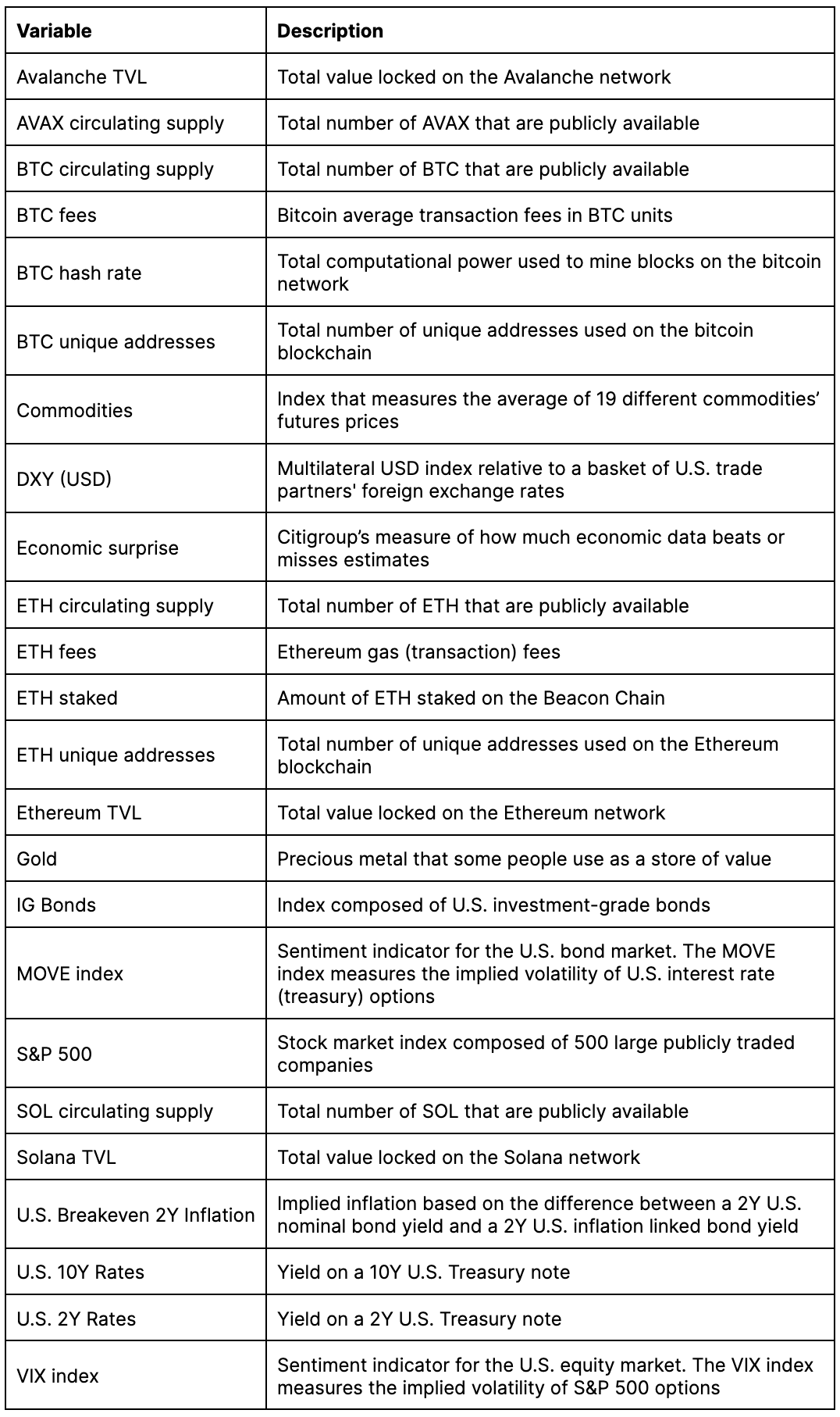
The inputs to our model include:

• broad macroeconomic variables like economic surprise indices for U.S., Europe and China; U.S. 2Y and 10Y Treasury rates as well as U.S. breakeven inflation
• other asset classes including the S&P 500, commodities, investment grade corporate bonds, DXY (multilateral USD index) and gold
• sentiment indicators like the VIX index (for stocks) and the MOVE index (for bonds)
• crypto specific factors like bitcoin hash rates, unique address counts, Ethereum gas fees, circulating supply, staked ETH and total value locked

Note that the ability to back test in this space is limited by a lack of available historical data. For example, the price history for SOL only goes back as far as March 2020 and for AVAX back to September 2020, while the total value locked on both networks was zero in the early part of 1Q21. This constrains the amount of viable data that can be used to test and train our ML model. Also complicating things is that because crypto markets run 24/7, we need to use the right timestamp on their prices corresponding to the end-of-day prices of other asset classes.

The importance of a given input or “feature” is defined here by its strength in explaining the observed price movements in BTC, ETH, SOL and AVAX. Notably, we employ a method known as Shapley Additive Explanations (SHAP) to quantify the relative importance of our inputs. The appeal of SHAP values is that the model results can be explained in a relatively straightforward way. SHAP values help us understand the impact of having a certain value for a given feature in comparison to the prediction we'd make if that feature took some baseline value.

SHAP values that tend towards zero reflect features of little predictive relevance in our model while values moving away from zero reflect features of increasingly higher importance. But what this measure is actually identifying are which inputs best refine (or “split”) our decision tree(s) along the most meaningful dimensions in order to learn the key relationships that could affect our predicted outcomes.